In mathematics, linear interpolation is a method of curve fitting using linear polynomials to construct new data points within the range of a discrete set of known data points.[1]

In [1]:

%matplotlib inline
%watermark -dtvmp numpy,matplotlib,pandas,cython

import matplotlib.pylab as plt
import lerp
from lerp import *

2017-10-12 22:57:48

CPython 3.6.2
IPython 6.1.0

numpy 1.13.1
matplotlib 2.0.2
pandas 0.20.3
cython 0.26.1

compiler   : GCC 4.2.1 Compatible Clang 4.0.1 (tags/RELEASE_401/final)
system     : Darwin
release    : 15.6.0
machine    : x86_64
processor  : i386
CPU cores  : 2
interpreter: 64bit

In [2]:

lerp.options.display.max_rows = 15

Usage¶

BreakPoints¶

In [3]:

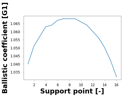
A = BreakPoints(d=[1.040, 1.051, 1.057, 1.063, 1.064, 1.067, 1.068, 1.068, 1.068, 1.066, 1.064,
                1.060, 1.056, 1.050, 1.042, 1.032], label="Ballistic coefficient", unit="G1")

Display in the notebook, integer above the value are helps for indexing purpose

In [4]:

Out[4]:

BreakPoints: Ballistic coefficient [G1]

0	1	2	3	4	5	6	7	8	9	10	11	12	13	...	15
1.04	1.051	1.057	1.063	1.064	1.067	1.068	1.068	1.068	1.066	1.064	1.06	1.056	1.05	...	1.032

In [5]:

A[6]

Out[5]:

1.0680000000000001

Get a plot with the plot() method

In [6]:

A.plot()

Out[6]:

[<matplotlib.lines.Line2D at 0x181b8a0400>]

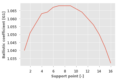
Not that fancy… you can set the ggplot style

In [7]:

plt.style.use('ggplot')
A.plot()

Out[7]:

[<matplotlib.lines.Line2D at 0x181ba223c8>]

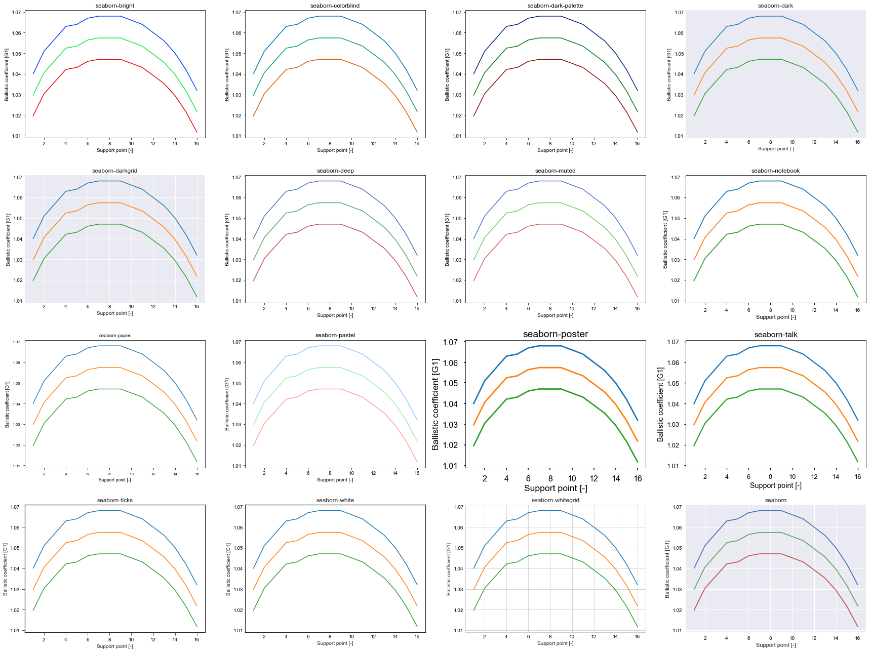
If you don’t like ggplot, choose one of the seaborn styles

In [8]:

import matplotlib.gridspec as gridspec
import matplotlib as mpl
styles = [_s for _s in plt.style.available if 'seaborn' in _s]
n = np.ceil(np.sqrt(len(styles))).astype(np.int)

gs = gridspec.GridSpec(n, n)

plt.figure(figsize=(24,18))

for i, s in enumerate(styles):
    mpl.rcParams.update(mpl.rcParamsDefault)
    plt.style.use(s)
    plt.subplot(gs[i])
    A.plot()
    (A / 1.01).plot()
    (A / 1.02).plot()
    plt.title(s)

plt.tight_layout()

mesh2d¶

From Ballistic coefficient article in Wikipedia.

Doppler radar measurement results for a lathe turned monolithic solid .50 BMG very-low-drag bullet (Lost River J40 13.0 millimetres (0.510 in), 50.1 grams (773 gr) monolithic solid bullet / twist rate 1:380 millimetres (15 in)) look like this:

In [9]:

BC = mesh2d(x=np.arange(500,2100,100), x_label="Range", x_unit="m",
            d=[1.040, 1.051, 1.057, 1.063, 1.064, 1.067, 1.068, 1.068, 1.068, 1.066, 1.064,
               1.060, 1.056, 1.050, 1.042, 1.032], label="Ballistic coefficient", unit="G1")

Display in the jupyter notebooks / ipython

In [10]:

BC

Out[10]:

mesh2d

	0	1	2	3	4	5	6	7	8	9	10	11	12	13	...	15
Range [m]	500	600	700	800	900	1000	1100	1200	1300	1400	1500	1600	1700	1800	...	2000
Ballistic coefficient [G1]	1.04	1.051	1.057	1.063	1.064	1.067	1.068	1.068	1.068	1.066	1.064	1.06	1.056	1.05	...	1.032

Interpolation

In [11]:

BC(501)

Out[11]:

1.04011

In [12]:

BC([501, 609, 2500])

Out[12]:

array([ 1.04011,  1.05154,  0.982  ])

Default : values are extrapolated

In [13]:

BC.interpolate([501, 609, 2500])

Out[13]:

array([ 1.04011,  1.05154,  1.032  ])

Interpolation is performed and boundaries values are kept

In [14]:

BC.options

Out[14]:

{'extrapolate': True, 'step': False}

In [15]:

BC.options['extrapolate']= False

This can be controled though the dict key extrapolate in options or interpolate method.

In [16]:

BC([501, 609, 2500])

Out[16]:

array([ 1.04011,  1.05154,  1.032  ])

In [17]:

BC.max()

Out[17]:

1.0680000000000001

In [18]:

BC.max(argwhere=True)

Out[18]:

(1100, 1.0680000000000001)

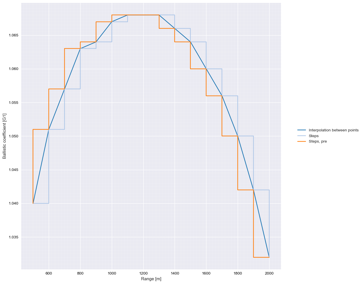
Plot as steps

I like the color from vega

In [19]:

from cycler import cycler
category20 = cycler('color', ['#1f77b4', '#aec7e8', '#ff7f0e',
                              '#ffbb78', '#2ca02c', '#98df8a',
                              '#d62728', '#ff9896', '#9467bd',
                              '#c5b0d5', '#8c564b', '#c49c94',
                              '#e377c2', '#f7b6d2', '#7f7f7f',
                              '#c7c7c7', '#bcbd22', '#dbdb8d',
                              '#17becf', '#9edae5'])

plt.style.use('seaborn-darkgrid')
plt.rc('axes', prop_cycle=category20)

In [20]:

plt.figure(figsize=(10,10))

BC.plot(label="Interpolation between points")
BC.steps.plot(label="Steps")
BC.steps.plot(where="pre", label="Steps, pre")

plt.graphpaper(dx=200, dy=0.005)
plt.legend(bbox_to_anchor=(1.05, 0.5), loc='center left', facecolor="white", frameon=False)
plt.tight_layout()

Slicing

In [21]:

BC[2:4]

Out[21]:

mesh2d

	0	1
Range [m]	700	800
Label [unit]	1.057	1.063

Breakpoints strictly monotone, reverse order has no effect

In [22]:

BC[::-1]

Out[22]:

mesh2d

	0	1	2	3	4	5	6	7	8	9	10	11	12	13	...	15
Range [m]	500	600	700	800	900	1000	1100	1200	1300	1400	1500	1600	1700	1800	...	2000
Label [unit]	1.04	1.051	1.057	1.063	1.064	1.067	1.068	1.068	1.068	1.066	1.064	1.06	1.056	1.05	...	1.032

In [23]:

BC[6]

Out[23]:

(1100, 1.0680000000000001)

In [24]:

BC.x

Out[24]:

BreakPoints: Range [m]

0	1	2	3	4	5	6	7	8	9	10	11	12	13	...	15
500	600	700	800	900	1000	1100	1200	1300	1400	1500	1600	1700	1800	...	2000

In [25]:

BC(np.arange(500, 550, 10))

Out[25]:

array([ 1.04  ,  1.0411,  1.0422,  1.0433,  1.0444])

In [26]:

BC.resample(np.arange(500, 2000, 200))

Out[26]:

mesh2d

	0	1	2	3	4	5	6	7
Range [m]	500	700	900	1100	1300	1500	1700	1900
Ballistic coefficient [G1]	1.04	1.057	1.064	1.068	1.068	1.064	1.056	1.042

In [27]:

BC.steps(BC.x)

Out[27]:

array([ 1.04 ,  1.051,  1.057,  1.063,  1.064,  1.067,  1.068,  1.068,
        1.068,  1.066,  1.064,  1.06 ,  1.056,  1.05 ,  1.042,  1.032])

In [28]:

BC.__dict__

Out[28]:

{'_d': array([ 1.04 ,  1.051,  1.057,  1.063,  1.064,  1.067,  1.068,  1.068,
         1.068,  1.066,  1.064,  1.06 ,  1.056,  1.05 ,  1.042,  1.032]),
 '_options': {'extrapolate': False, 'step': False},
 '_steps': x = BreakPoints(d=[ 500,  600,  700,  800,  900, 1000, 1100, 1200, 1300, 1400,
              1500, 1600, 1700, 1800, 1900, 2000], label="Range", unit="m")
 d = array([ 1.04 ,  1.051,  1.057,  1.063,  1.064,  1.067,  1.068,  1.068,
         1.068,  1.066,  1.064,  1.06 ,  1.056,  1.05 ,  1.042,  1.032]),
 '_x': BreakPoints(d=[ 500,  600,  700,  800,  900, 1000, 1100, 1200, 1300, 1400,
              1500, 1600, 1700, 1800, 1900, 2000], label="Range", unit="m"),
 'label': 'Ballistic coefficient',
 'unit': 'G1'}

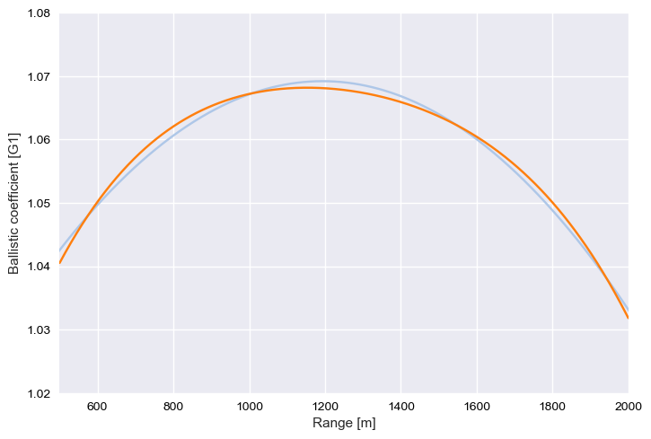
.polyfit(): how to get a polymesh object from discrete values

In [29]:

BC.plot("+")
BC.polyfit(degree=2).plot(xlim=[500,2000])
BC.polyfit(degree=4).plot(xlim=[500,2000], ylim=[1.02, 1.08])

In [30]:

BC.polyfit(degree=4)

Out[30]:

-3.5896443597682554e-14·x⁴ + 1.820225053584262e-10·x³ - 3.821239680082758e-07·x² + 0.00037528910653332015·x + 0.9278994701119253

In [31]:

from sklearn.metrics import r2_score

for i in range(10):
    print(i, r2_score(BC.d, BC.polyfit(degree=i)(BC.x).d))

0 0.0
1 0.0698263920953
2 0.988101760851
3 0.988408030976
4 0.997727098729
5 0.998238919776
6 0.998565636158
7 0.998569159428
8 0.998610724807
9 0.998652377691

.add()

In [32]:

# prepare some data
x = [1, 2, 3, 4, 5]
y = [6, 7, 2, 4, 5]
test2 = mesh2d(x, y)
x2 = np.arange(0,60)
test = mesh2d(x2, np.sin(x2), x_label="Mon label", unit="%")

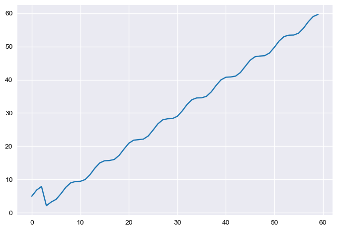
In [33]:

(test + test2)

Out[33]:

mesh2d

	0	1	2	3	4	5	6	7	8	9	10	11	12	13	...	59
Label [unit]	0	1	2	3	4	5	6	7	8	9	10	11	12	13	...	59
Label [%]	5.0	6.84147098481	7.90929742683	2.14112000806	3.24319750469	4.04107572534	5.7205845018	7.65698659872	8.98935824662	9.41211848524	9.45597888911	10.0000097934	11.463427082	13.4201670368	...	59.6367380071

In [34]:

test[:4]

Out[34]:

mesh2d

	0	1	2	3
Mon label [unit]	0	1	2	3
Label [unit]	0.0	0.841470984808	0.909297426826	0.14112000806

In [35]:

test[-3:] + test[:4]

Out[35]:

mesh2d

	0	1	2	3	4	5	6
Label [unit]	0	1	2	3	57	58	59
Label [unit]	-31.2961851364	-29.8980062588	-29.2734719239	-29.4849414499	-40.90429585	-41.115765376	-42.2400774357

In [36]:

(test + test2).plot()

Out[36]:

[<matplotlib.lines.Line2D at 0x181d938240>]

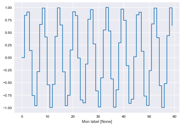
In [37]:

test.steps.plot()

Out[37]:

[<matplotlib.lines.Line2D at 0x181c046630>]

In [38]:

test

Out[38]:

mesh2d

	0	1	2	3	4	5	6	7	8	9	10	11	12	13	...	59
Mon label [unit]	0	1	2	3	4	5	6	7	8	9	10	11	12	13	...	59
Label [%]	0.0	0.841470984808	0.909297426826	0.14112000806	-0.756802495308	-0.958924274663	-0.279415498199	0.656986598719	0.989358246623	0.412118485242	-0.544021110889	-0.999990206551	-0.536572918	0.420167036827	...	0.636738007139

In [39]:

test.resample(np.linspace(0,60,100))

Out[39]:

mesh2d

	0	1	2	3	4	5	6	7	8	9	10	11	12	13	...	99
Mon label [unit]	0.0	0.606060606061	1.21212121212	1.81818181818	2.42424242424	3.0303030303	3.63636363636	4.24242424242	4.84848484848	5.45454545455	6.06060606061	6.66666666667	7.27272727273	7.87878787879	...	60.0
Label [%]	0.0	0.509982415035	0.855858411903	0.896965346459	0.58340397644	0.113910235231	-0.430285221356	-0.805801714546	-0.92829976264	-0.650056648998	-0.222663855961	0.344852566413	0.747633411784	0.94907077415	...	0.280603366194

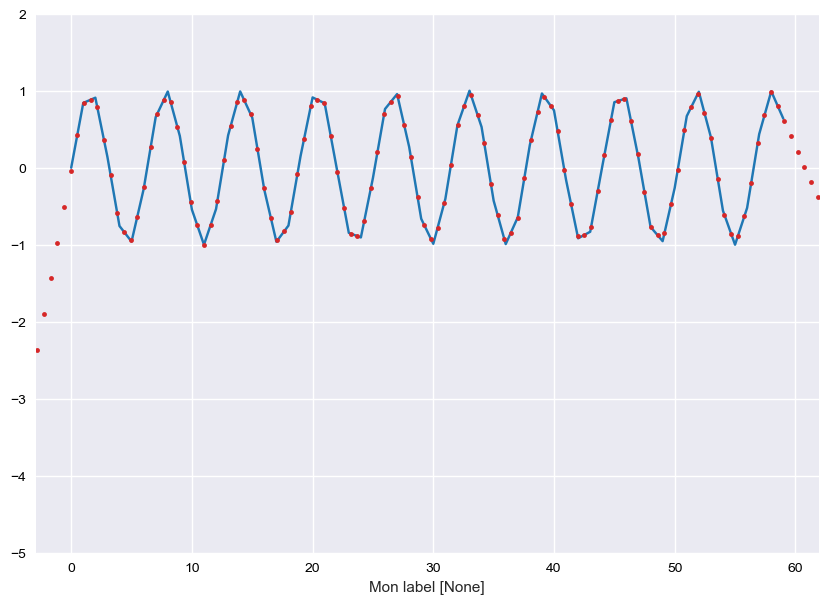
In [40]:

plt.figure(figsize=(12,7))
test.plot()
newX = np.linspace(-10,100,200)
test.resample(newX).plot('.', c=category20.by_key()['color'][6], lw=0.1)
plt.ylim(-5, 2)

Out[40]:

(-5, 2)

Not implemented

In [41]:

test + test2.steps

Out[41]:

mesh2d

	0	1	2	3	4	5	6	7	8	9	10	11	12	13	...	59
Label [unit]	0	1	2	3	4	5	6	7	8	9	10	11	12	13	...	59
Label [%]	5.0	6.84147098481	7.90929742683	2.14112000806	3.24319750469	4.04107572534	5.7205845018	7.65698659872	8.98935824662	9.41211848524	9.45597888911	10.0000097934	11.463427082	13.4201670368	...	59.6367380071

In [42]:

test.steps([-10, 2.3, 3, 3.1, 59, 58.9, 90])

Out[42]:

array([ -8.41470985,   0.6788442 ,   0.14112001,   0.05132776,
         0.63673801,   0.67235147, -10.40343586])

In [43]:

test.steps

Out[43]:

mesh2d

	0	1	2	3	4	5	6	7	8	9	10	11	12	13	...	59
Mon label [unit]	0	1	2	3	4	5	6	7	8	9	10	11	12	13	...	59
Label [%]	0.0	0.841470984808	0.909297426826	0.14112000806	-0.756802495308	-0.958924274663	-0.279415498199	0.656986598719	0.989358246623	0.412118485242	-0.544021110889	-0.999990206551	-0.536572918	0.420167036827	...	0.636738007139

In [44]:

test.diff(n=1)

Out[44]:

mesh2d

	0	1	2	3	4	5	6	7	8	9	10	11	12	13	...	58
Mon label [unit]	0	1	2	3	4	5	6	7	8	9	10	11	12	13	...	58
Label [unit]	0.841470984808	0.0678264420178	-0.768177418766	-0.897922503368	-0.202121779355	0.679508776464	0.936402096918	0.332371647905	-0.577239761382	-0.956139596131	-0.455969095661	0.46341728855	0.956739954827	0.570440318868	...	-0.356134640945

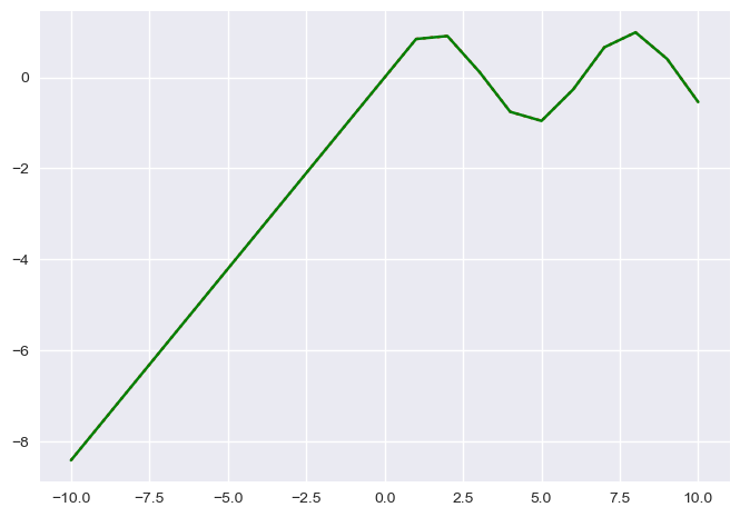
In [45]:

#plt.plot(test.X, test.Y, c="b")
newX = np.arange(-10, 10, 0.001)
plt.plot(newX, test(newX), ":r")
plt.plot(newX, test.steps(newX), "-g")

Out[45]:

[<matplotlib.lines.Line2D at 0x181ba962e8>]

In [46]:

test.steps(newX)

Out[46]:

array([-8.41470985, -8.41386838, -8.41302691, ..., -0.54115269,
       -0.54210883, -0.54306497])

In [47]:

import random
from numba import jit

N = 200
myMesh = mesh2d(np.arange(N)*5, [random.uniform(2.5, 10.0) for i in range(N)], x_label="MON Label")

In [48]:

@jit
def _extrapolate(self, X):
    """
    """
    if X <= self.x[0]:
        res = self.d[0] + (X - self.x[0]) *\
            (self.d[1] - self.d[0]) / (self.x[1] - self.x[0])
    elif X >= self.x[-1]:
        res = self.d[-1] + (x - self.x[-1]) *\
            (self.d[-1] - self.d[-2]) / (self.x[-1] - self.x[-2])
    else:
        res = np.interp(X, self.x, self.d)
    return res

In [49]:

%timeit myMesh.extrapolate(255)

21.7 µs ± 915 ns per loop (mean ± std. dev. of 7 runs, 10000 loops each)

In [50]:

%timeit _extrapolate(myMesh, 255)

The slowest run took 5.50 times longer than the fastest. This could mean that an intermediate result is being cached.
94.3 µs ± 87.9 µs per loop (mean ± std. dev. of 7 runs, 1 loop each)

In [51]:

np.diff(test2.d) / np.diff(test2.x)

Out[51]:

BreakPoints: Label [unit]

0	1	2	3
1.0	-5.0	2.0	1.0

%timeit myMesh.resample(np.arange(-1000, 2000))%timeit np.interp(np.arange(-1000, 2000), myMesh.x, myMesh.d)%timeit np.interp(range(3000), myMesh.x, myMesh.d)%timeit myMesh(np.arange(-10000, 200000))%timeit [myMesh(x) for x in np.arange(-10000, 200000)]

mesh3d¶

In [52]:

m3d = mesh3d(x=np.arange(10), x_label="X", x_unit="X unit",
             y=np.arange(10), y_label="Y", y_unit="Y unit",
             d=np.random.random((10,10)), label="data", unit="data unit")

In [53]:

lerp.options.display.max_rows = 15

In [54]:

m3d

Out[54]:

mesh3d: data [data unit]

			Y [Y unit]
			0	1	2	3	4	5	6	7	8	9
			0	1	2	3	4	5	6	7	8	9
X [X unit]	0	0	0.434870352236	0.231482446855	0.323554590807	0.194513188669	0.548793345442	0.96149870994	0.844978297764	0.0228477172479	0.897581614385	0.374790493167
	1	1	0.437402209826	0.587596826678	0.791935900857	0.797250085103	0.172353816711	0.307922572235	0.892314438845	0.0389261541275	0.152285593713	0.668586250984
	2	2	0.239566423457	0.117757222828	0.0778158520051	0.408587080639	0.575914282062	0.615422273431	0.0794269216571	0.241520040366	0.576474949269	0.428839200808
	3	3	0.401880455557	0.323199273872	0.457562472467	0.0141568154629	0.227149073091	0.465886627968	0.103495434375	0.432788853357	0.543142697729	0.624016873678
	4	4	0.997010442368	0.580724632779	0.78920553766	0.433053909205	0.899167356663	0.136601551671	0.321671088169	0.0719736098203	0.873654825756	0.0908232066389
	5	5	0.839283164546	0.0983105134967	0.336623680254	0.922124339553	0.000231907931159	0.299444518868	0.14549982256	0.941861267225	0.0852897382606	0.806634210453
	6	6	0.329042869533	0.733084098255	0.36561023492	0.837637339275	0.358071677098	0.819752114767	0.835915137057	0.612484846397	0.665516593392	0.917622397535
	7	7	0.321520224323	0.882292871723	0.131471934025	0.0638956540853	0.0575484791685	0.313598324598	0.932679129866	0.582086515852	0.271956817773	0.322686998655
	8	8	0.687338866596	0.342367197937	0.00667948763791	0.878436083913	0.103669100142	0.78076360356	0.794991264318	0.100103968489	0.498882006535	0.515767614048
	9	9	0.662384794299	0.984440654163	0.994469603672	0.611867904981	0.852381106735	0.846679230244	0.689709361867	0.136597804809	0.376000954499	0.960696980125

In [55]:

m3d(4.5, 5.7)

Out[55]:

0.22891672933562421

Interpolation

In [56]:

m3d(3.5, 5.6)

Out[56]:

0.24804759269057369

Call method default : extrapolation above boundaries

In [57]:

m3d(9.1,9.4)

Out[57]:

1.2617807437078306

As far mesh2d, can be set with options attributes or method call .interpolate

In [58]:

m3d.options

Out[58]:

{'extrapolate': True}

In [59]:

m3d.interpolate(9.1,9.4)

Out[59]:

0.9606969801252196

In [60]:

m3d(x=3.5)

Out[60]:

mesh2d

	0	1	2	3	4	5	6	7	8	9
Y [Y unit]	0	1	2	3	4	5	6	7	8	9
Label [unit]	0.699445448962	0.451961953325	0.623384005064	0.223605362334	0.563158214877	0.301244089819	0.212583261272	0.252381231588	0.708398761743	0.357420040158

Slicing

In [61]:

m3d[3:6]

Out[61]:

mesh3d: data [data unit]

			Y [Y unit]
			0	1	2	3	4	5	6	7	8	9
			0	1	2	3	4	5	6	7	8	9
X [X unit]	0	3	0.401880455557	0.323199273872	0.457562472467	0.0141568154629	0.227149073091	0.465886627968	0.103495434375	0.432788853357	0.543142697729	0.624016873678
	1	4	0.997010442368	0.580724632779	0.78920553766	0.433053909205	0.899167356663	0.136601551671	0.321671088169	0.0719736098203	0.873654825756	0.0908232066389
	2	5	0.839283164546	0.0983105134967	0.336623680254	0.922124339553	0.000231907931159	0.299444518868	0.14549982256	0.941861267225	0.0852897382606	0.806634210453

Garbage after that point

In [62]:

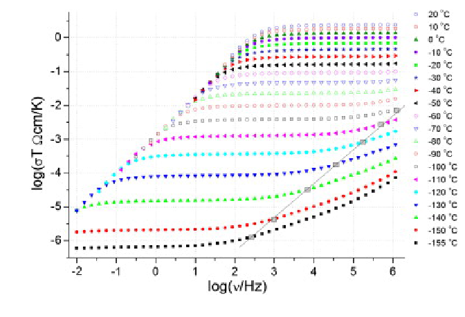
from scipy import misc
from scipy import ndimage
# http://www.ndt.net/article/wcndt00/papers/idn360/idn360.htm

from PIL import Image
from urllib.request import urlopen
import io

URL = 'https://www.researchgate.net/profile/Robert_Dinnebier/publication/268693474/figure/fig5/AS:268859169046548@1441112429791/Log-log-plot-of-ionic-conductivity-times-temperature-versus-frequency-measured-at.png'

with urlopen(URL) as url:
    im = misc.imread(io.BytesIO(url.read()))

# face = misc.imread(f)

In [63]:

plt.imshow(im, cmap=plt.cm.gray, vmin=30, vmax=200)
plt.axis('off')
# plt.contour(im, [50, 200])

Out[63]:

(-0.5, 388.5, 259.5, -0.5)

In [64]:

sx = ndimage.sobel(im, axis=0, mode='constant')
sy = ndimage.sobel(im, axis=1, mode='constant')
sob = np.hypot(sx, sy)

In [65]:

sx = ndimage.sobel(im, axis=0, mode='constant')

import numpy as np import matplotlib.pyplot as plt from scipy import interpolate x = np.array([[0.12, 0.11, 0.1, 0.09, 0.08], [0.13, 0.12, 0.11, 0.1, 0.09], [0.15, 0.14, 0.12, 0.11, 0.1], [0.17, 0.15, 0.14, 0.12, 0.11], [0.19, 0.17, 0.16, 0.14, 0.12], [0.22, 0.19, 0.17, 0.15, 0.13], [0.24, 0.22, 0.19, 0.16, 0.14], [0.27, 0.24, 0.21, 0.18, 0.15], [0.29, 0.26, 0.22, 0.19, 0.16]]) y = np.array([[71.64, 78.52, 84.91, 89.35, 97.58], [66.28, 73.67, 79.87, 85.36, 93.24], [61.48, 69.31, 75.36, 81.87, 89.35], [57.61, 65.75, 71.7, 79.1, 86.13], [55.12, 63.34, 69.32, 77.29, 83.88], [54.58, 62.54, 68.7, 76.72, 82.92], [56.58, 63.87, 70.3, 77.69, 83.53], [61.67, 67.79, 74.41, 80.43, 85.86], [70.08, 74.62, 80.93, 85.06, 89.84]]) plt.figure(figsize = (9, 9)) plt.subplot(111) for i in range(5): x_val = np.linspace(x[0, i], x[-1, i], 100) x_int = np.interp(x_val, x[:, i], y[:, i]) tck = interpolate.splrep(x[:, i], y[:, i], k = 2, s = 4) y_int = interpolate.splev(x_val, tck, der = 0) plt.plot(x[:, i], y[:, i], linestyle = '', marker = 'o') plt.plot(x_val, y_int, linestyle = ':', linewidth = 0.25, color = 'black') plt.xlabel('X') plt.ylabel('Y') plt.show()from scipy.interpolate import dfitpack, fitpackdef extrapolate(self, X, Y): if X <= self.X[0]: iX = 0 elif X >= self.X[-1]: iX = -2 else: iX = np.searchsorted(self.X, X) - 1 if Y <= self.Y[0]: iY = 0 elif Y >= self.Y[-1]: iY = -2 else: iY = np.searchsorted(self.Y, Y) - 1 Z1 = self.W[iX, iY] + (self.W[iX, iY+1] - self.W[iX, iY]) * \ (Y - self.Y[iY]) / (self.Y[iY+1] - self.Y[iY]) Z2 = self.W[iX+1, iY] + (self.W[iX+1, iY+1] - self.W[iX+1, iY]) * \ (Y - self.Y[iY]) / (self.Y[iY+1] - self.Y[iY]) return Z1 + (Z2 - Z1) * (X - self.X[iX]) / (self.X[iX+1] - self.X[iX])def interpolate(self, X, Y): if X <= self.X[0]: return np.interp(Y, self.Y, self.W[0]) elif X >= self.X[-1]: return np.interp(Y, self.Y, self.W[-1]) else: iX = np.searchsorted(self.X, X) - 1 if Y <= self.Y[0]: return np.interp(X, self.X, self.W[:,0]) elif Y >= self.Y[-1]: return np.interp(X, self.X, self.W[:,-1]) else: iY = np.searchsorted(self.Y, Y) - 1 Z1 = self.W[iX, iY] + (self.W[iX, iY+1] - self.W[iX, iY]) * \ (Y - self.Y[iY]) / (self.Y[iY+1] - self.Y[iY]) Z2 = self.W[iX+1, iY] + (self.W[iX+1, iY+1] - self.W[iX+1, iY]) * \ (Y - self.Y[iY]) / (self.Y[iY+1] - self.Y[iY]) return Z1 + (Z2 - Z1) * (X - self.X[iX]) / (self.X[iX+1] - self.X[iX])%timeit interpolate(m3d, 15,1)np.diff(m3d.W[1:3,2:4], axis=1)%timeit np.diff(m3d.W[1:3,2:4], axis=1)%timeit m3d.W[1:3,3] - m3d.W[1:3,2]np.diff(m3d.W[1:3,2:4], axis=0)m3d = mesh3d(np.arange(100),np.arange(50),np.random.random((50,100)))def extrapolate(self, X, Y): iX = 0 iY = 0 if X <= self.X[0]: iX = 0 elif X >= self.X[-1]: iX = -2 else: iX = np.where(self.X < X)[0][-1] if Y <= self.Y[0]: iY = 0 elif Y >= self.Y[-1]: iY = -2 else: iY = np.where(self.Y < Y)[0][-1] Z1 = self.W[iY, iX] + (self.W[iY, iX+1] - self.W[iY, iX]) * \ (X - self.X[iX]) / (self.X[iX+1] - self.X[iX]) Z2 = self.W[iY+1, iX] + (self.W[iY+1, iX+1] - self.W[iY+1, iX]) * \ (X - self.X[iX]) / (self.X[iX+1] - self.X[iX]) return Z1 + (Z2 - Z1) * (Y - self.Y[iY]) / (self.Y[iY+1] - self.Y[iY]) def extrapolate1(self, _X, _Y): xNew = np.searchsorted(self.X, _X).clip(1, len(self.X)-1).astype(int) yNew = np.searchsorted(self.Y, _Y).clip(1, len(self.Y)-1).astype(int) # 4. Calculate the slope of regions that each X value falls in. xLo, xHi = xNew - 1, xNew yLo, yHi = yNew - 1, yNew x11 = self.X[xLo] x12 = self.X[xHi] y11 = self.Y[yLo] y21 = self.Y[yHi] w11 = self.W[:,xLo] w12 = self.W[:,xHi] # Note that the following two expressions rely on the specifics of the # broadcasting semantics. xSlope = (w12 - w11) / (x12 - x11) # 5. Calculate the actual value for each entry in X. yNew = xSlope * (_X - x11) + w11 w11 = yNew[yLo] w21 = yNew[yHi] ySlope = (w21 - w11) / (y21 - y11) yNew = ySlope * (_Y - y11) + w11 return np.array(yNew) def extrapolate2(self, X, Y): iX = -2 if X >= self.X[-1] else \ np.searchsorted(self.X, X).clip(1, len(self.X)-1).astype(int) - 1 iY = -2 if Y >= self.Y[-1] else \ np.searchsorted(self.Y, Y).clip(1, len(self.Y)-1).astype(int) - 1 Z1 = self.W[iY, iX] + (self.W[iY, iX+1] - self.W[iY, iX]) * \ (X - self.X[iX]) / (self.X[iX+1] - self.X[iX]) Z2 = self.W[iY+1, iX] + (self.W[iY+1, iX+1] - self.W[iY+1, iX]) * \ (X - self.X[iX]) / (self.X[iX+1] - self.X[iX]) return Z1 + (Z2 - Z1) * (Y - self.Y[iY]) / (self.Y[iY+1] - self.Y[iY])def extrapolate3(self, X, Y): gc.disable() st = time.time() if X <= self.X[0]: iX = 0 elif X >= self.X[-1]: iX = -2 else: iX = np.searchsorted(self.X, X) - 1 if Y <= self.Y[0]: iY = 0 elif Y >= self.Y[-1]: iY = -2 else: iY = np.searchsorted(self.Y, Y) - 1 Z1 = self.W[iY, iX] + (self.W[iY, iX+1] - self.W[iY, iX]) * \ (X - self.X[iX]) / (self.X[iX+1] - self.X[iX]) Z2 = self.W[iY+1, iX] + (self.W[iY+1, iX+1] - self.W[iY+1, iX]) * \ (X - self.X[iX]) / (self.X[iX+1] - self.X[iX]) return Z1 + (Z2 - Z1) * (Y - self.Y[iY]) / (self.Y[iY+1] - self.Y[iY])New meshfrom functools import singledispatchclass newmesh(np.ndarray): def __new__(cls, data=None, label=None, unit=None): # We first cast to be our class type # np.asfarray([], dtype='float64') @singledispatch def myArray(o): if o is None: o = [] # Will call directly __array_finalize__ obj = np.asarray(o).flatten().view(cls) obj.label = label obj.unit = unit return obj @myArray.register(mesh1d) def _(o): if label is not None: o.label = label if unit is not None: o.unit = unit return o return myArray(data) # see InfoArray.__array_finalize__ for comments def __array_finalize__(self, obj): """ :type obj: object """ self.unit = getattr(obj, 'unit', None) self.label = getattr(obj, 'label', None) @property def d(self): return self[0] @d.setter def d(self, obj): self[0] = objtest = newmesh([1, 3, 4])test.d = 5test.flags

[1] lerp article on Wikipedia

Table Of Contents

Usage¶

BreakPoints¶

mesh2d¶

.polyfit(): how to get a polymesh object from discrete values

.add()

mesh3d¶